Indexing for AI Workloads: What Changes When Vectors Enter the Mix
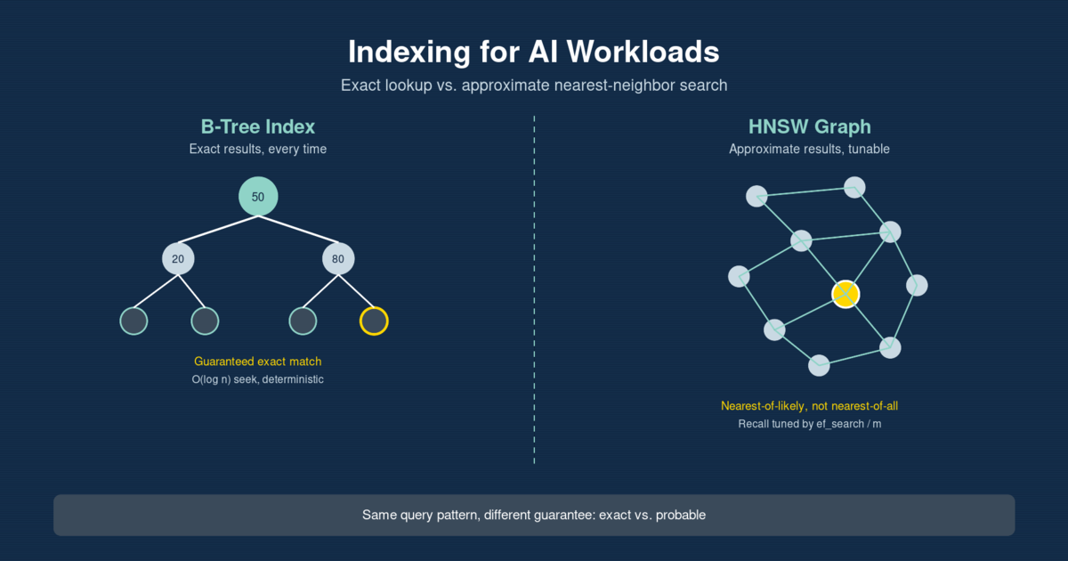
Adding a vector column to an existing database breaks a promise every DBA has relied on since B-trees became the default: that an index returns the correct rows, every time, in a predictable amount of time. HNSW and IVFFlat, the two index types behind vector search, are approximate by design – they trade a guaranteed-correct answer for a fast one, and that single shift changes how you build, tune, size, and monitor these indexes compared to everything else in the database.
Why this matters now
Vector columns are no longer a specialized add-on. PostgreSQL 18 merged native vector types and HNSW/IVFFlat indexing directly into core rather than leaving it to the pgvector extension, and SQL Server 2025 reached general availability in November 2025 with a native VECTOR type and DiskANN indexing built in (Microsoft Azure SQL Devs’ Corner). Retrieval-augmented generation, semantic search, and recommendation features are landing in the same schema as the OLTP tables that back a company’s core application – which means the DBA who’s spent a career tuning B-tree and columnstore indexes is now also responsible for a completely different index family with different failure modes.
Key takeaways
- HNSW and IVFFlat are approximate nearest-neighbor (ANN) indexes – unlike a B-tree, they don’t guarantee the exact correct result set, only a statistically likely one
- Recall is a tunable dial, not a fixed property:
ef_searchcontrols the query-time speed/accuracy tradeoff without a rebuild, whilemandef_constructionare baked in at build time - HNSW graphs are held largely in memory; at 1M vectors they typically consume 3-4x the memory of an IVFFlat index of the same data
- Filtering a vector search (
WHEREclauses alongside similarity search) needs a different strategy than filtering a normal query – pre-filtering and post-filtering perform very differently depending on selectivity - AI can flag when a vector index’s recall has silently drifted below a threshold; deciding whether to rebuild, re-tune, or re-quantize stays a human call
No more exact answers
A B-tree seek on an indexed column returns every matching row, full stop. An HNSW or IVFFlat query returns the rows the graph thinks are closest – and depending on how the index is tuned, it can miss the true nearest neighbor entirely. This isn’t a bug; it’s the entire point. Finding the exact nearest neighbor among millions of high-dimensional vectors is too slow to be useful, so both index types walk a graph or a set of clusters looking for a “good enough” answer fast.
That tradeoff is controlled by parameters that don’t have an equivalent in relational indexing:
m(HNSW) – the maximum number of graph connections per node, set at build time. Highermmeans a denser graph, better recall, more memory, and slower builds. The pgvector default is 16.ef_construction(HNSW) – how large a candidate list the index considers while building each node’s connections. Must be at least 2xm. Higher values produce a better graph but take longer to build.ef_search(HNSW) – the size of the candidate list at query time. This is the parameter most worth tuning after deployment, because it can be changed per-query without touching the index at all. Widening it recovers recall at the cost of latency.
In a representative benchmark on a 10-million-row, 128-dimension dataset, ef_search=128 returns better than 99% recall in under 5 milliseconds, while dropping to ef_search=64 lands around 97% recall at roughly 2 milliseconds. Neither number is wrong – they’re two different points on the same curve, and choosing between them is a product decision, not a database one. A support-ticket similarity search can usually tolerate 97%. A compliance-related legal document search probably can’t.
The memory bill nobody warns you about
B-tree indexes are disk-resident by default and cached opportunistically. HNSW is built to live in memory – the graph traversal that makes it fast depends on avoiding page faults during the walk. A rough sizing formula for planning capacity: N x D x 4 bytes x 2, where N is the row count, D is the vector dimension, and the trailing 2 accounts for graph-edge overhead. At 5 million vectors and 1536 dimensions – a typical OpenAI embedding size – that’s 8 to 16 GB of working memory for the index alone, before accounting for the base table or anything else running on the instance.
That number also explains why build time can blow up unexpectedly. If PostgreSQL’s maintenance_work_mem (64 MB by default) is too small to hold the graph during construction, the build spills to disk and can run 10 to 50 times slower (dbi-services pgvector guide). This is the single most common “why is my index build hanging” complaint on new vector deployments, and the fix is a session-level memory setting, not a code change.
Quantization techniques – binary quantization, half-precision floats, statistical binary quantization – are the current answer to the memory problem. Vendor benchmarks report footprint reductions of up to 12x with minimal recall loss, though those figures are worth verifying against your own data rather than taking at face value (Tiger Data pgvectorscale benchmark).
What changes about inserts and maintenance
IVFFlat clusters the data once, at build time, and doesn’t rebalance on its own. Heavy insert activity after the initial build drifts the data away from those original clusters, and recall degrades quietly until someone runs a REINDEX. HNSW updates its graph incrementally as rows are inserted, which avoids the drift problem, but each insert costs more than an HNSW graph search plus edge rewiring – noticeably more expensive than a B-tree insert, and worth accounting for in write-heavy workloads.
Neither index type follows the maintenance rhythm a DBA already knows from ALTER INDEX REBUILD or REORGANIZE. Recall degradation on an ANN index doesn’t throw an error or show up in a corruption check – it just returns worse answers, and the only way to catch it is to measure recall against a held-out ground-truth set on a schedule.
Filtering: the part that surprises people first
Nearly every real vector search also needs a WHERE clause – restrict results to one tenant, one date range, one category. Two baseline strategies exist, and picking the wrong one for the data’s selectivity produces either a slow query or an incomplete result set:
- Pre-filtering: apply the
WHEREclause first, then brute-force the similarity search across the survivors. Fast when the filter is highly selective (few rows match); collapses back toward a full scan when it isn’t. - Post-filtering: run the ANN search first, then discard rows that fail the filter. Fast when the filter is broad, but can under-return results entirely when the filter is narrow and the top-K candidates mostly get discarded.
Newer engines are starting to close this gap. pgvector added iterative scans that keep searching until enough post-filter rows survive, and academic work on filter-aware index structures (ACORN, Filtered-DiskANN) reports 2.6x to 3x throughput gains over naive pre/post filtering by building filter-awareness into the graph itself (arXiv: Filtered Approximate Nearest Neighbor Search in Vector Databases). If your workload is mostly filtered vector search rather than pure similarity search, this is worth checking for on whatever platform you’re evaluating.
What this means for the team running the database
None of this replaces relational indexing knowledge – it sits alongside it. A schema that mixes transactional tables with vector columns needs someone who understands both B-tree seek plans and HNSW recall curves, and right now that’s rarely the same person by default. The practical starting point is treating ef_search as a per-query, per-workload tuning lever rather than a fixed setting, budgeting memory for the vector index as its own line item rather than assuming it shares headroom with everything else, and putting a recall-measurement job on a schedule the same way query-plan regression checks already run.
This connects directly to what we’ve covered on semantic readiness and database performance diagnosis – vector indexing sits at the intersection of both.
If your database is carrying both relational and vector workloads and nobody’s measured recall drift lately, get in touch – this is exactly the kind of readiness gap that’s cheap to close before it shows up as a production incident.
Ivan Lima is a data engineer specializing in database modernization for AI systems. Get in touch if your database needs to be ready for what’s next.